9 Joining Data with dplyr
https://learn.datacamp.com/courses/joining-data-with-dplyr
##
## Attaching package: 'dplyr'
## The following objects are masked from 'package:stats':
##
## filter, lag## The following objects are masked from 'package:base':
##
## intersect, setdiff, setequal, union## ── Attaching packages ───────────────────────── tidyverse 1.3.0 ──## ✓ ggplot2 3.3.3 ✓ purrr 0.3.4
## ✓ tibble 3.0.3 ✓ stringr 1.4.0
## ✓ tidyr 1.1.2 ✓ forcats 0.5.0
## ✓ readr 1.3.1## ── Conflicts ──────────────────────────── tidyverse_conflicts() ──
## x dplyr::filter() masks stats::filter()
## x dplyr::lag() masks stats::lag()9.1 Joining Tables
The inner_join verb: We can use the inner join verb to merge two datasets. The inner_join is the key to bring tables together. To use it, you need to provide the two tables that must be joined and the columns on which they should be joined.
data_1 <- gapminder %>% select(country, continent, gdpPercap) %>% mutate(index_continent = row_number())
data_2 <- gapminder %>% select(country, year, lifeExp) %>% mutate(index_country = row_number())

data_1
## # A tibble: 1,704 x 4
## country continent gdpPercap index_continent
## <fct> <fct> <dbl> <int>
## 1 Afghanistan Asia 779. 1
## 2 Afghanistan Asia 821. 2
## 3 Afghanistan Asia 853. 3
## 4 Afghanistan Asia 836. 4
## 5 Afghanistan Asia 740. 5
## 6 Afghanistan Asia 786. 6
## 7 Afghanistan Asia 978. 7
## 8 Afghanistan Asia 852. 8
## 9 Afghanistan Asia 649. 9
## 10 Afghanistan Asia 635. 10
## # … with 1,694 more rows## # A tibble: 1,704 x 4
## country year lifeExp index_country
## <fct> <int> <dbl> <int>
## 1 Afghanistan 1952 28.8 1
## 2 Afghanistan 1957 30.3 2
## 3 Afghanistan 1962 32.0 3
## 4 Afghanistan 1967 34.0 4
## 5 Afghanistan 1972 36.1 5
## 6 Afghanistan 1977 38.4 6
## 7 Afghanistan 1982 39.9 7
## 8 Afghanistan 1987 40.8 8
## 9 Afghanistan 1992 41.7 9
## 10 Afghanistan 1997 41.8 10
## # … with 1,694 more rows## # A tibble: 1,704 x 7
## country.x continent gdpPercap index_continent country.y year lifeExp
## <fct> <fct> <dbl> <int> <fct> <int> <dbl>
## 1 Afghanistan Asia 779. 1 Afghanistan 1952 28.8
## 2 Afghanistan Asia 821. 2 Afghanistan 1957 30.3
## 3 Afghanistan Asia 853. 3 Afghanistan 1962 32.0
## 4 Afghanistan Asia 836. 4 Afghanistan 1967 34.0
## 5 Afghanistan Asia 740. 5 Afghanistan 1972 36.1
## 6 Afghanistan Asia 786. 6 Afghanistan 1977 38.4
## 7 Afghanistan Asia 978. 7 Afghanistan 1982 39.9
## 8 Afghanistan Asia 852. 8 Afghanistan 1987 40.8
## 9 Afghanistan Asia 649. 9 Afghanistan 1992 41.7
## 10 Afghanistan Asia 635. 10 Afghanistan 1997 41.8
## # … with 1,694 more rowsWe can add the suffix arguement to change names of the variables with same name.
data_joint <- data_1 %>%
  inner_join(data_2, by = c("index_continent" = "index_country"), suffix = c("_main", "_notRequired"))

data_joint
## # A tibble: 1,704 x 7
## country_main continent gdpPercap index_continent country_notRequ… year
## <fct> <fct> <dbl> <int> <fct> <int>
## 1 Afghanistan Asia 779. 1 Afghanistan 1952
## 2 Afghanistan Asia 821. 2 Afghanistan 1957
## 3 Afghanistan Asia 853. 3 Afghanistan 1962
## 4 Afghanistan Asia 836. 4 Afghanistan 1967
## 5 Afghanistan Asia 740. 5 Afghanistan 1972
## 6 Afghanistan Asia 786. 6 Afghanistan 1977
## 7 Afghanistan Asia 978. 7 Afghanistan 1982
## 8 Afghanistan Asia 852. 8 Afghanistan 1987
## 9 Afghanistan Asia 649. 9 Afghanistan 1992
## 10 Afghanistan Asia 635. 10 Afghanistan 1997
## # … with 1,694 more rows, and 1 more variable: lifeExp <dbl>final_data <- data_joint %>% select(country = country_main, continent, year, lifeExp, gdpPercap)
final_data## # A tibble: 1,704 x 5
## country continent year lifeExp gdpPercap
## <fct> <fct> <int> <dbl> <dbl>
## 1 Afghanistan Asia 1952 28.8 779.
## 2 Afghanistan Asia 1957 30.3 821.
## 3 Afghanistan Asia 1962 32.0 853.
## 4 Afghanistan Asia 1967 34.0 836.
## 5 Afghanistan Asia 1972 36.1 740.
## 6 Afghanistan Asia 1977 38.4 786.
## 7 Afghanistan Asia 1982 39.9 978.
## 8 Afghanistan Asia 1987 40.8 852.
## 9 Afghanistan Asia 1992 41.7 649.
## 10 Afghanistan Asia 1997 41.8 635.
## # … with 1,694 more rows9.2 Left and Right Joins
An inner join() only keep observations that appear in both tables.But if want to keep all the observations of the first table (left table) while joining we use the left_join verb. Similarly, if want to keep all the observations of the second table (right table) while joining we use the right_join verb.
inventory_parts_joined <- inventories %>%
  inner_join(inventory_parts, by = c("id" = "inventory_id")) %>%
  select(-id, -version) %>%
  arrange(desc(quantity))

head(inventory_parts_joined)
## # A tibble: 6 x 4
## set_num part_num color_id quantity
## <chr> <chr> <dbl> <dbl>
## 1 40179-1 3024 72 900
## 2 40179-1 3024 15 900
## 3 40179-1 3024 0 900
## 4 40179-1 3024 71 900
## 5 40179-1 3024 14 900
## 6 k34434-1 3024 15 810batmobile <- inventory_parts_joined %>%
filter(set_num == "7784-1") %>%
select(-set_num)
batwing <- inventory_parts_joined %>%
filter(set_num == "70916-1") %>%
select(-set_num)
batmobile## # A tibble: 173 x 3
## part_num color_id quantity
## <chr> <dbl> <dbl>
## 1 3023 72 62
## 2 2780 0 28
## 3 50950 0 28
## 4 3004 71 26
## 5 43093 1 25
## 6 3004 0 23
## 7 3010 0 21
## 8 30363 0 21
## 9 32123b 14 19
## 10 3622 0 18
## # … with 163 more rows## # A tibble: 309 x 3
## part_num color_id quantity
## <chr> <dbl> <dbl>
## 1 3023 0 22
## 2 3024 0 22
## 3 3623 0 20
## 4 11477 0 18
## 5 99207 71 18
## 6 2780 0 17
## 7 3666 0 16
## 8 22385 0 14
## 9 3710 0 14
## 10 99563 0 13
## # … with 299 more rowsbatmobile %>%
left_join(batwing, by = c("part_num", "color_id"), suffix = c("_batmobile", "_batwing"))## # A tibble: 173 x 4
## part_num color_id quantity_batmobile quantity_batwing
## <chr> <dbl> <dbl> <dbl>
## 1 3023 72 62 NA
## 2 2780 0 28 17
## 3 50950 0 28 2
## 4 3004 71 26 2
## 5 43093 1 25 6
## 6 3004 0 23 4
## 7 3010 0 21 NA
## 8 30363 0 21 NA
## 9 32123b 14 19 NA
## 10 3622 0 18 2
## # … with 163 more rows#Filter where Quantity_batmobile = NA
batmobile %>%
right_join(batwing, by = c("part_num", "color_id"), suffix = c("_batmobile", "_batwing")) %>%
filter(is.na(quantity_batmobile))## # A tibble: 267 x 4
## part_num color_id quantity_batmobile quantity_batwing
## <chr> <dbl> <dbl> <dbl>
## 1 3023 0 NA 22
## 2 11477 0 NA 18
## 3 99207 71 NA 18
## 4 3666 0 NA 16
## 5 22385 0 NA 14
## 6 3710 0 NA 14
## 7 99563 0 NA 13
## 8 10247 72 NA 12
## 9 2877 72 NA 12
## 10 61409 72 NA 12
## # … with 257 more rows#Replace NA with 0
batmobile %>%
right_join(batwing, by = c("part_num", "color_id"), suffix = c("_batmobile", "_batwing")) %>%
replace_na(list(quantity_batmobile = 0))## # A tibble: 312 x 4
## part_num color_id quantity_batmobile quantity_batwing
## <chr> <dbl> <dbl> <dbl>
## 1 2780 0 28 17
## 2 50950 0 28 2
## 3 3004 71 26 2
## 4 43093 1 25 6
## 5 3004 0 23 4
## 6 3622 0 18 2
## 7 4286 0 16 1
## 8 3039 0 12 2
## 9 4274 71 12 7
## 10 3001 0 11 4
## # … with 302 more rowsWe can join a table to itself.
themes <- readRDS("themes.rds")

themes %>%
    # Inner join the themes table
    inner_join(themes, by = c("id" = "parent_id"), suffix = c("_parent", "_child")) %>%
    # Filter for the "Harry Potter" parent name
    filter(name_parent == "Harry Potter")
## # A tibble: 6 x 5
## id name_parent parent_id id_child name_child
## <dbl> <chr> <dbl> <dbl> <chr>
## 1 246 Harry Potter NA 247 Chamber of Secrets
## 2 246 Harry Potter NA 248 Goblet of Fire
## 3 246 Harry Potter NA 249 Order of the Phoenix
## 4 246 Harry Potter NA 250 Prisoner of Azkaban
## 5 246 Harry Potter NA 251 Sorcerer's Stone
## 6 246 Harry Potter NA 667 Fantastic Beaststhemes %>%
# Left join the themes table to its own children
left_join(themes, by = c("id" = "parent_id"), suffix = c("_parent", "_child")) %>%
# Filter for themes that have no child themes
filter(is.na(name_child))## # A tibble: 586 x 5
## id name_parent parent_id id_child name_child
## <dbl> <chr> <dbl> <dbl> <chr>
## 1 2 Arctic Technic 1 NA <NA>
## 2 3 Competition 1 NA <NA>
## 3 4 Expert Builder 1 NA <NA>
## 4 6 Airport 5 NA <NA>
## 5 7 Construction 5 NA <NA>
## 6 8 Farm 5 NA <NA>
## 7 9 Fire 5 NA <NA>
## 8 10 Harbor 5 NA <NA>
## 9 11 Off-Road 5 NA <NA>
## 10 12 Race 5 NA <NA>
## # … with 576 more rows9.3 Full, Semi, and Anti Joins
We use the full_join verb when we want to keep all observations from both the data sets we are joining.
batmobile %>%
full_join(batwing, by = c("part_num", "color_id"), suffix = c("_batmobile", "_batwing"))
## # A tibble: 440 x 4
## part_num color_id quantity_batmobile quantity_batwing
## <chr> <dbl> <dbl> <dbl>
## 1 3023 72 62 NA
## 2 2780 0 28 17
## 3 50950 0 28 2
## 4 3004 71 26 2
## 5 43093 1 25 6
## 6 3004 0 23 4
## 7 3010 0 21 NA
## 8 30363 0 21 NA
## 9 32123b 14 19 NA
## 10 3622 0 18 2
## # … with 430 more rowsThe semi- and atin- join verbs:
A filtering join keeps or removes observations from the first table but it doesn’t add new variables.
The semi join asks the question “What observations in X are also in Y?”
## # A tibble: 45 x 3
##    part_num color_id quantity
##    <chr>       <dbl>    <dbl>
##  1 2780            0       28
##  2 50950           0       28
##  3 3004           71       26
##  4 43093           1       25
##  5 3004            0       23
##  6 3622            0       18
##  7 4286            0       16
##  8 3039            0       12
##  9 4274           71       12
## 10 3001            0       11
## # … with 35 more rows
The anti join asks the question “What observations in X are NOT in Y?”
## # A tibble: 128 x 3
##    part_num color_id quantity
##    <chr>       <dbl>    <dbl>
##  1 3023           72       62
##  2 3010            0       21
##  3 30363           0       21
##  4 32123b         14       19
##  5 50950         320       18
##  6 6541            0       18
##  7 3040b           0       14
##  8 3298            0       14
##  9 3660            0       14
## 10 42022           0       14
## # … with 118 more rows
Visualizing set differences:
Aggregating sets into color:
## `summarise()` ungrouping output (override with `.groups` argument)## # A tibble: 12 x 2
## color_id total
## <dbl> <dbl>
## 1 0 543
## 2 1 33
## 3 4 16
## 4 14 20
## 5 15 16
## 6 36 15
## 7 57 8
## 8 71 202
## 9 72 160
## 10 182 8
## 11 297 4
## 12 320 27## `summarise()` ungrouping output (override with `.groups` argument)## # A tibble: 20 x 2
## color_id total
## <dbl> <dbl>
## 1 0 418
## 2 1 45
## 3 4 81
## 4 14 22
## 5 15 22
## 6 19 10
## 7 25 1
## 8 34 3
## 9 36 9
## 10 46 21
## 11 47 4
## 12 52 4
## 13 57 3
## 14 70 16
## 15 71 158
## 16 72 213
## 17 78 3
## 18 80 4
## 19 179 1
## 20 182 14colors <- readRDS("colors.rds")
colors_joint <- batmobile_colors %>%
full_join(batwing_colors, by = "color_id", suffix = c("_batmobile", "_batwing")) %>%
replace_na(list(total_batmobile = 0, total_batwing = 0)) %>%
inner_join(colors, by = c("color_id" = "id")) %>%
mutate(total_batmobile = total_batmobile / sum(total_batmobile),
total_batwing = total_batwing / sum(total_batwing),
difference = total_batmobile - total_batwing)library(ggplot2)
library(forcats)
color_palette <- setNames(colors_joint$rgb, colors_joint$name)
colors_joint %>%
mutate(name = fct_reorder(name, difference)) %>%
ggplot(aes(name, difference, fill = name)) +
geom_col() +
coord_flip()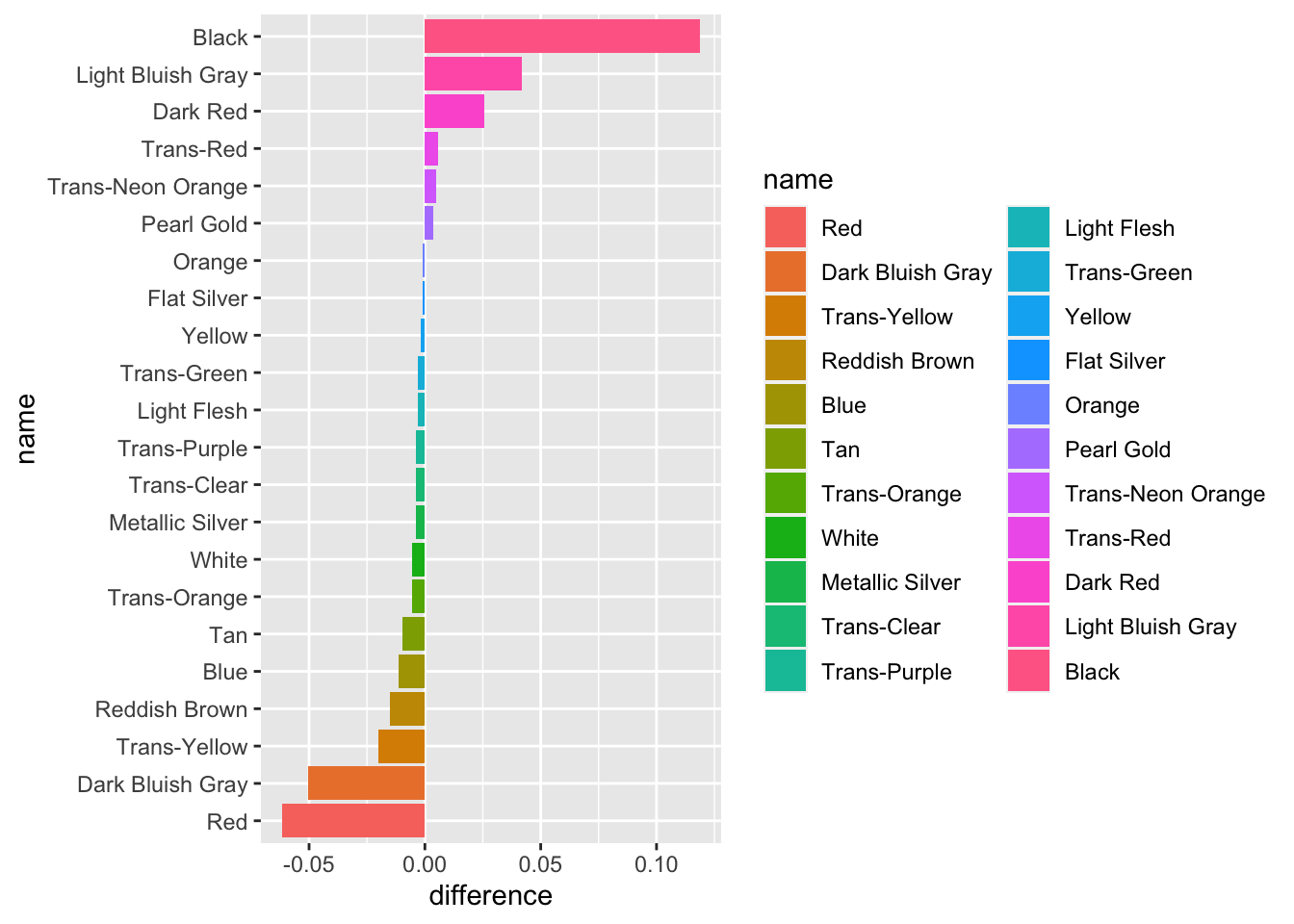
9.4 Case Study: Joins on Stack Overflow Data
question_tags <- readRDS("question_tags.rds")
questions <- readRDS("questions.rds")
tags <- readRDS("tags.rds")
question_with_tags <- questions %>%
inner_join(question_tags, by = c("id" = "question_id")) %>%
inner_join(tags, by = c("tag_id" = "id"))
question_with_tags## # A tibble: 497,153 x 5
## id creation_date score tag_id tag_name
## <int> <date> <int> <dbl> <chr>
## 1 22557677 2014-03-21 1 18 regex
## 2 22557677 2014-03-21 1 139 string
## 3 22557677 2014-03-21 1 16088 time-complexity
## 4 22557677 2014-03-21 1 1672 backreference
## 5 22558084 2014-03-21 2 6419 time-series
## 6 22558084 2014-03-21 2 92764 panel-data
## 7 22558395 2014-03-21 2 5569 function
## 8 22558395 2014-03-21 2 134 sorting
## 9 22558395 2014-03-21 2 9412 vectorization
## 10 22558395 2014-03-21 2 18621 operator-precedence
## # … with 497,143 more rows# Replace the NAs in the tag_name column
questions %>%
left_join(question_tags, by = c("id" = "question_id")) %>%
left_join(tags, by = c("tag_id" = "id")) %>%
replace_na(list(tag_name = "only-r"))## # A tibble: 545,694 x 5
## id creation_date score tag_id tag_name
## <int> <date> <int> <dbl> <chr>
## 1 22557677 2014-03-21 1 18 regex
## 2 22557677 2014-03-21 1 139 string
## 3 22557677 2014-03-21 1 16088 time-complexity
## 4 22557677 2014-03-21 1 1672 backreference
## 5 22557707 2014-03-21 2 NA only-r
## 6 22558084 2014-03-21 2 6419 time-series
## 7 22558084 2014-03-21 2 92764 panel-data
## 8 22558395 2014-03-21 2 5569 function
## 9 22558395 2014-03-21 2 134 sorting
## 10 22558395 2014-03-21 2 9412 vectorization
## # … with 545,684 more rowsquestion_with_tags %>%
# Group by tag_name
group_by(tag_name) %>%
# Get mean score and num_questions
summarize(score = mean(score),
num_questions = n()) %>%
# Sort num_questions in descending order
arrange(desc(num_questions))## `summarise()` ungrouping output (override with `.groups` argument)## # A tibble: 7,840 x 3
## tag_name score num_questions
## <chr> <dbl> <int>
## 1 ggplot2 2.61 28228
## 2 dataframe 2.31 18874
## 3 shiny 1.45 14219
## 4 dplyr 1.95 14039
## 5 plot 2.24 11315
## 6 data.table 2.97 8809
## 7 matrix 1.66 6205
## 8 loops 0.743 5149
## 9 regex 2 4912
## 10 function 1.39 4892
## # … with 7,830 more rowsThe bind_rows verb:
Instead of joining the tables, if we want to stack one table on top of another, we use the bind_rows verb.
answers <- readRDS("answers (1).rds")

questions_type <- questions %>% mutate(type = "question")

answers_type <-  answers %>% mutate(type = "answer")

posts <- bind_rows(questions_type, answers_type)##
## Attaching package: 'lubridate'## The following objects are masked from 'package:base':
##
## date, intersect, setdiff, unionquestions_answers_year <- posts %>%
mutate(year = year(creation_date)) %>%
count(year, type)
ggplot(questions_answers_year, aes(year,n, color = type)) +
geom_line()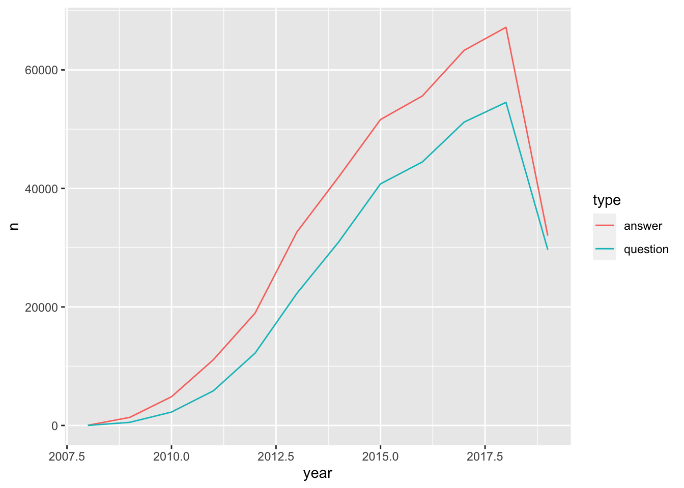
# Combine the two tables into posts_with_tags
posts_with_tags <- bind_rows(question_with_tags %>% mutate(type = "question"),
                              answers %>% mutate(type = "answer"))

# Add a year column, then aggregate by type, year, and tag_name
posts_with_tags %>%
  mutate(year = year(creation_date)) %>%
  count(type, year, tag_name)
## # A tibble: 29,983 x 4
## type year tag_name n
## <chr> <dbl> <chr> <int>
## 1 answer 2008 <NA> 27
## 2 answer 2009 <NA> 1361
## 3 answer 2010 <NA> 4847
## 4 answer 2011 <NA> 11079
## 5 answer 2012 <NA> 18967
## 6 answer 2013 <NA> 32652
## 7 answer 2014 <NA> 41953
## 8 answer 2015 <NA> 51630
## 9 answer 2016 <NA> 55601
## 10 answer 2017 <NA> 63306
## # … with 29,973 more rows