4 Intro to the Tidyverse
https://learn.datacamp.com/courses/introduction-to-the-tidyverse
4.1 Data wrangling
First, we need to install/load 2 packages - i) gapminder & ii) dplyr
We can then use glimpse/summary or simply gapminder itself to see the sumarry of the data set.
## ── Attaching packages ───────────────────────── tidyverse 1.3.0 ──## ✓ ggplot2 3.3.3 ✓ purrr 0.3.4
## ✓ tibble 3.0.3 ✓ dplyr 1.0.2
## ✓ tidyr 1.1.2 ✓ stringr 1.4.0
## ✓ readr 1.3.1 ✓ forcats 0.5.0## ── Conflicts ──────────────────────────── tidyverse_conflicts() ──
## x dplyr::filter() masks stats::filter()
## x dplyr::lag() masks stats::lag()## Rows: 1,704
## Columns: 6
## $ country <fct> Afghanistan, Afghanistan, Afghanistan, Afghanistan, Afghani…
## $ continent <fct> Asia, Asia, Asia, Asia, Asia, Asia, Asia, Asia, Asia, Asia,…
## $ year <int> 1952, 1957, 1962, 1967, 1972, 1977, 1982, 1987, 1992, 1997,…
## $ lifeExp <dbl> 28.801, 30.332, 31.997, 34.020, 36.088, 38.438, 39.854, 40.…
## $ pop <int> 8425333, 9240934, 10267083, 11537966, 13079460, 14880372, 1…
## $ gdpPercap <dbl> 779.4453, 820.8530, 853.1007, 836.1971, 739.9811, 786.1134,…Filter Verb:
The filter verb is used to make subsets of data from a data frame. It uses the “pipe” operator - %>% which takes whatever is before it and feeds it to whatever is after it.
## # A tibble: 12 x 6
##    country    continent  year lifeExp       pop gdpPercap
##    <fct>      <fct>     <int>   <dbl>     <int>     <dbl>
##  1 Bangladesh Asia       1952    37.5  46886859      684.
##  2 Bangladesh Asia       1957    39.3  51365468      662.
##  3 Bangladesh Asia       1962    41.2  56839289      686.
##  4 Bangladesh Asia       1967    43.5  62821884      721.
##  5 Bangladesh Asia       1972    45.3  70759295      630.
##  6 Bangladesh Asia       1977    46.9  80428306      660.
##  7 Bangladesh Asia       1982    50.0  93074406      677.
##  8 Bangladesh Asia       1987    52.8 103764241      752.
##  9 Bangladesh Asia       1992    56.0 113704579      838.
## 10 Bangladesh Asia       1997    59.4 123315288      973.
## 11 Bangladesh Asia       2002    62.0 135656790     1136.
## 12 Bangladesh Asia       2007    64.1 150448339     1391.
The Arrange Verb: The arrange verb helps us sort data in ascending and descending order.
We can combine filter and arrange whenever we need.
Mutate Verb:
The mutate verb is used to change or add variables to datasets. Inside the mutate verb, what’s on the right of the = sign is the change and what’s on the left is what’s being replaced.
To change a variable:
To add a new variable:
Combining mutate,filter, arrange:
4.2 Data visualization
To create a scatter plot, we use the following code after installing ggplot2
gapminder_1952 <- gapminder %>% filter(year == 1952)

ggplot(gapminder_1952, aes(x = pop, y = gdpPercap)) +
  geom_point()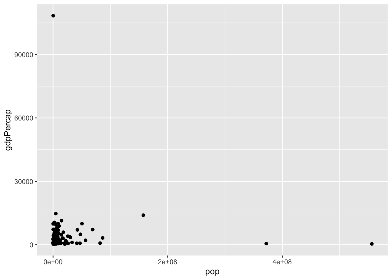
Log Scales :
If a variable is spread over several orders of magnitude, we can use a log scale. FOllowing is how a scatterplot looks before and after a using log scale respectively.
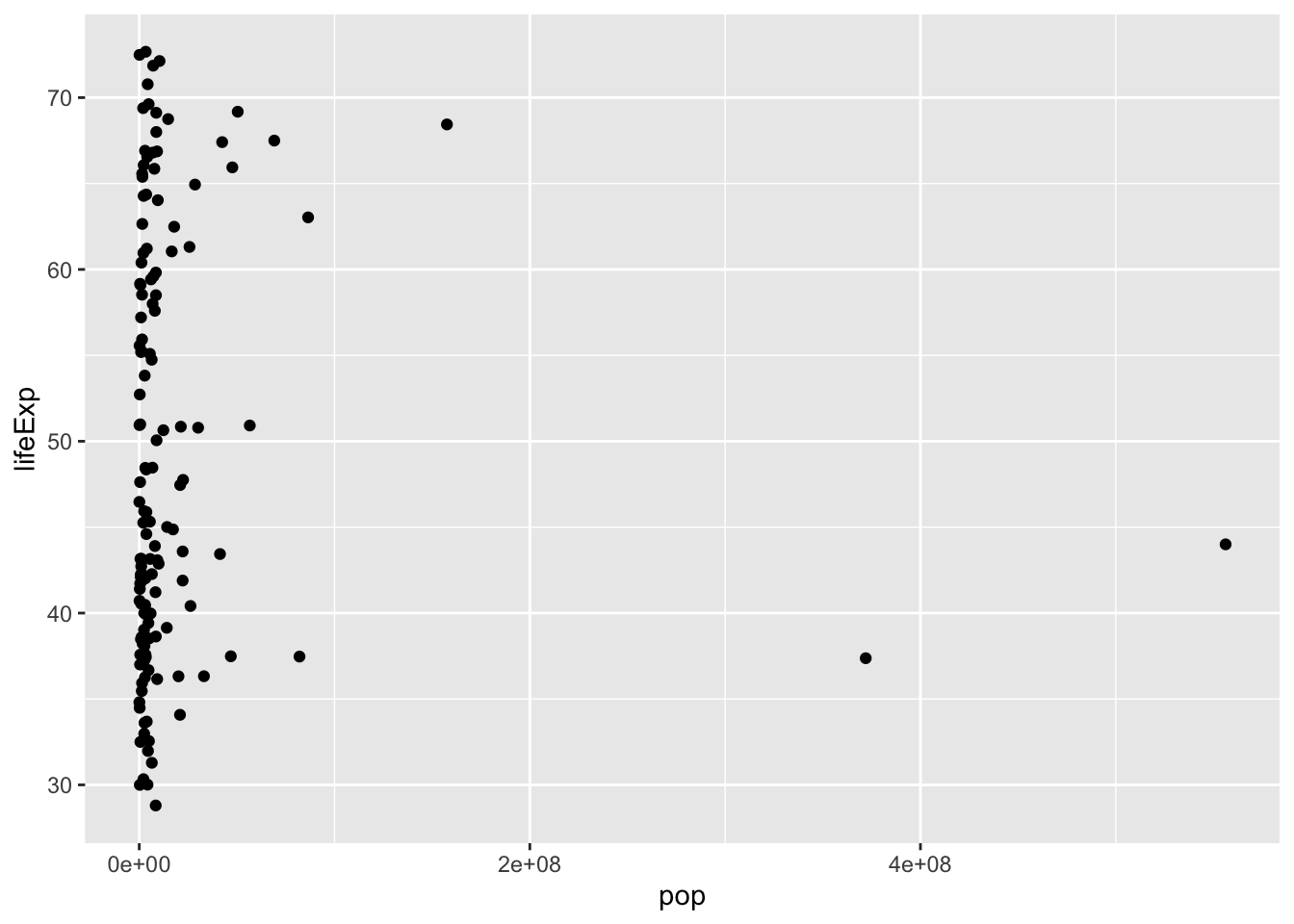
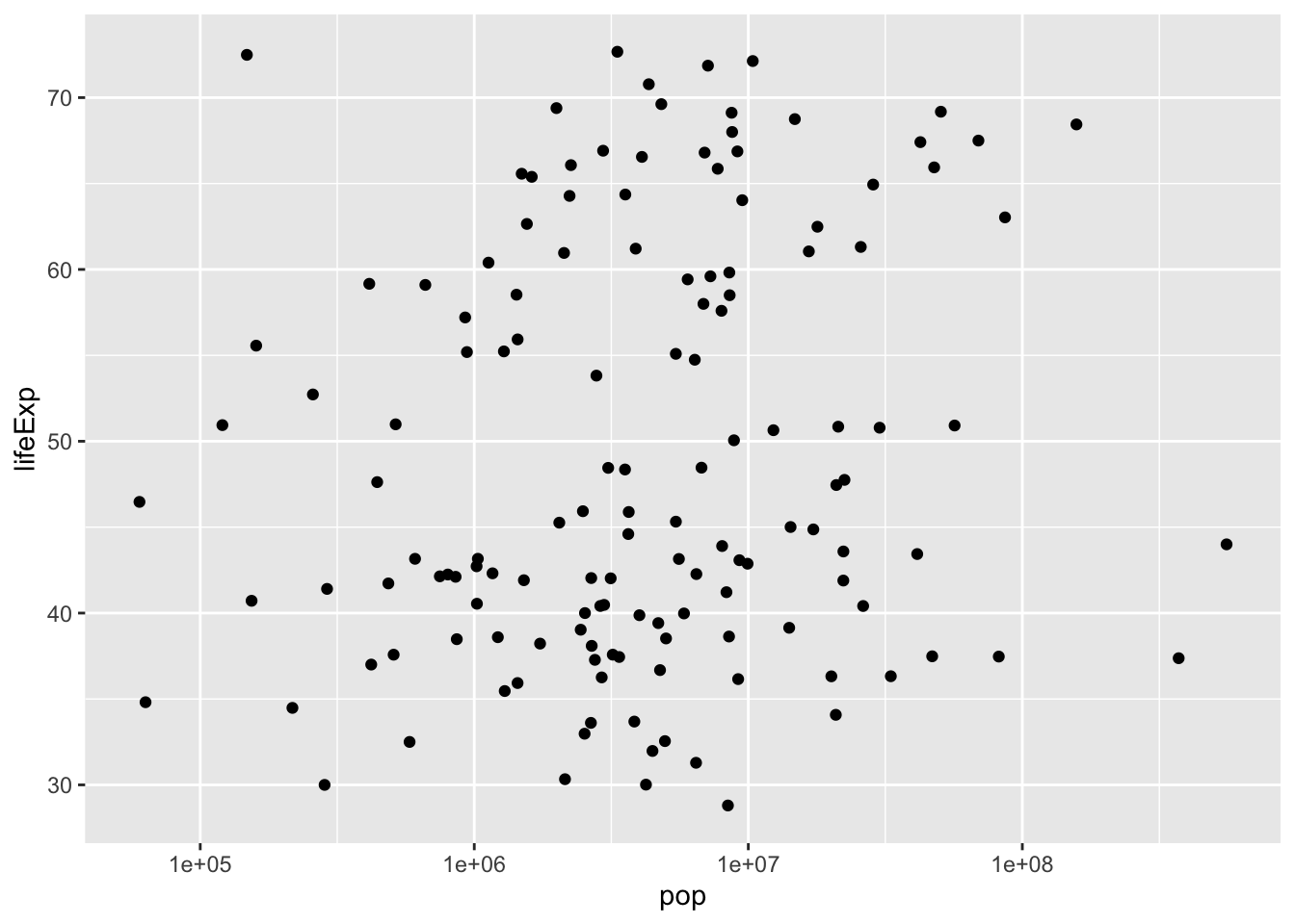
We can also change the y axis using a log scale:
ggplot(gapminder_1952, aes(x = pop, y = gdpPercap)) +
geom_point() +
scale_x_log10() +
scale_y_log10()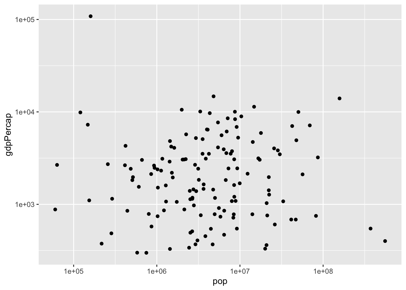
Additional Aesthetics:
We can add the color and size aesthetics to separate different variables.
ggplot(gapminder_1952, aes(x = pop, y = lifeExp, color = continent, size = gdpPercap)) +
geom_point() +
scale_x_log10() +
scale_y_log10()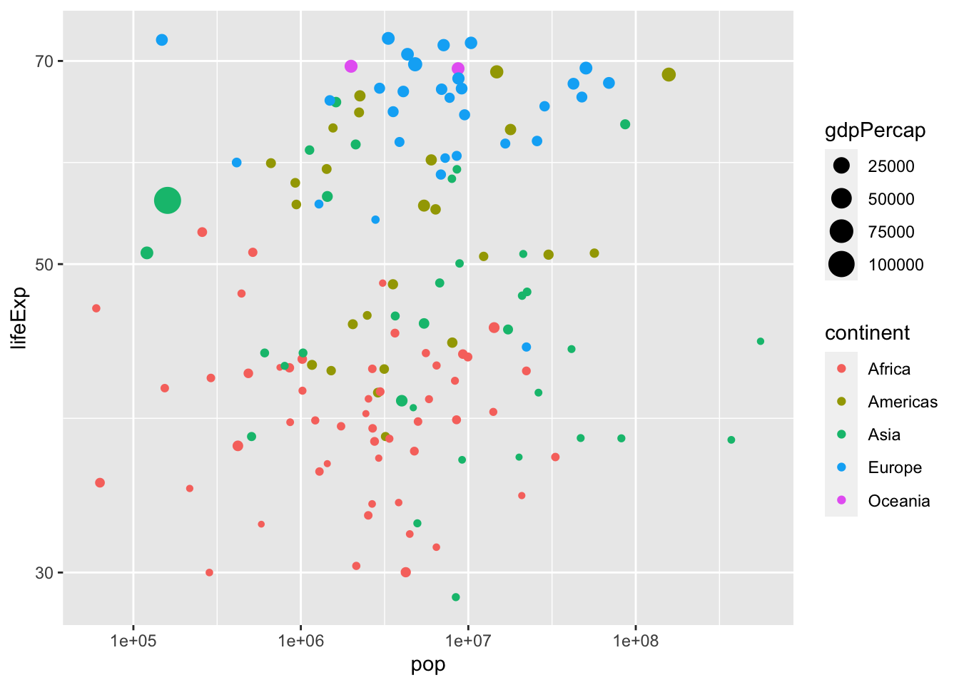 Faceting:
We can use faceting to divide a graph into subplots based on one of its variables, such as the continent. ~ symbol resembles ‘by’.
ggplot(gapminder_1952, aes(x = pop, y = lifeExp)) +
geom_point() +
scale_x_log10() +
facet_wrap (~ continent)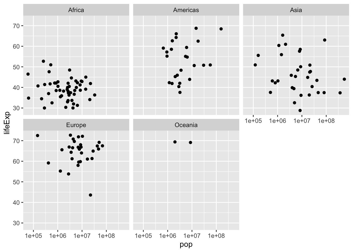 ## Grouping and summarizing
Summarize Verb :
We can use the summarize verb to summarize many observation into a single data point.
median_overall <-  gapminder %>%
  summarize(medianLifeExp = median(lifeExp))

mediun_1957 <- gapminder %>% filter(year == 1957) %>%
    summarize(medianLifeExp = median(lifeExp))
The summarize() verb also allows us to summarize multiple variables at once.
gapminder %>% filter(year == 1957) %>%
    summarize(medianLifeExp = median(lifeExp),
    maxGdpPercap = max(gdpPercap))
## # A tibble: 1 x 2
## medianLifeExp maxGdpPercap
## <dbl> <dbl>
## 1 48.4 113523.The Group_by Verb:
We can use the group_by verb along with the summarize verb to summarize data according to all the data pertaining to each value of of the variable it is being grouped by.
## `summarise()` ungrouping output (override with `.groups` argument)## # A tibble: 12 x 3
## year meanLifeExp totalPop
## <int> <dbl> <dbl>
## 1 1952 49.1 2406957150
## 2 1957 51.5 2664404580
## 3 1962 53.6 2899782974
## 4 1967 55.7 3217478384
## 5 1972 57.6 3576977158
## 6 1977 59.6 3930045807
## 7 1982 61.5 4289436840
## 8 1987 63.2 4691477418
## 9 1992 64.2 5110710260
## 10 1997 65.0 5515204472
## 11 2002 65.7 5886977579
## 12 2007 67.0 6251013179We can also perform multiple summarize verbs under one group by verb.
gapminder %>%
    group_by(year) %>%
    summarize(medianLifeExp = median(lifeExp),
              maxGdpPercap = max(gdpPercap))
## `summarise()` ungrouping output (override with `.groups` argument)## # A tibble: 12 x 3
## year medianLifeExp maxGdpPercap
## <int> <dbl> <dbl>
## 1 1952 45.1 108382.
## 2 1957 48.4 113523.
## 3 1962 50.9 95458.
## 4 1967 53.8 80895.
## 5 1972 56.5 109348.
## 6 1977 59.7 59265.
## 7 1982 62.4 33693.
## 8 1987 65.8 31541.
## 9 1992 67.7 34933.
## 10 1997 69.4 41283.
## 11 2002 70.8 44684.
## 12 2007 71.9 49357.We can use the filter, group_by and summarize verbs together :
gapminder %>%
    filter(year == 1957) %>%
    group_by(continent) %>%
    summarize(medianLifeExp = median(lifeExp),
              maxGdpPercap = max(gdpPercap))
## `summarise()` ungrouping output (override with `.groups` argument)## # A tibble: 5 x 3
## continent medianLifeExp maxGdpPercap
## <fct> <dbl> <dbl>
## 1 Africa 40.6 5487.
## 2 Americas 56.1 14847.
## 3 Asia 48.3 113523.
## 4 Europe 67.6 17909.
## 5 Oceania 70.3 12247.We can group by multiple variables before sumarizing.
by_year_continent <- gapminder %>%
    group_by(continent,year) %>%
    summarize(medianLifeExp = median(lifeExp),
              maxGdpPercap = max(gdpPercap))
## `summarise()` regrouping output by 'continent' (override with `.groups` argument)## # A tibble: 60 x 4
## # Groups: continent [5]
## continent year medianLifeExp maxGdpPercap
## <fct> <int> <dbl> <dbl>
## 1 Africa 1952 38.8 4725.
## 2 Africa 1957 40.6 5487.
## 3 Africa 1962 42.6 6757.
## 4 Africa 1967 44.7 18773.
## 5 Africa 1972 47.0 21011.
## 6 Africa 1977 49.3 21951.
## 7 Africa 1982 50.8 17364.
## 8 Africa 1987 51.6 11864.
## 9 Africa 1992 52.4 13522.
## 10 Africa 1997 52.8 14723.
## # … with 50 more rowsVisualizing summarized data:
We can show separate trends in a same graph.
ggplot(by_year_continent, aes(x = year, y = maxGdpPercap, color = continent)) +
geom_point() +
expand_limits(y=0)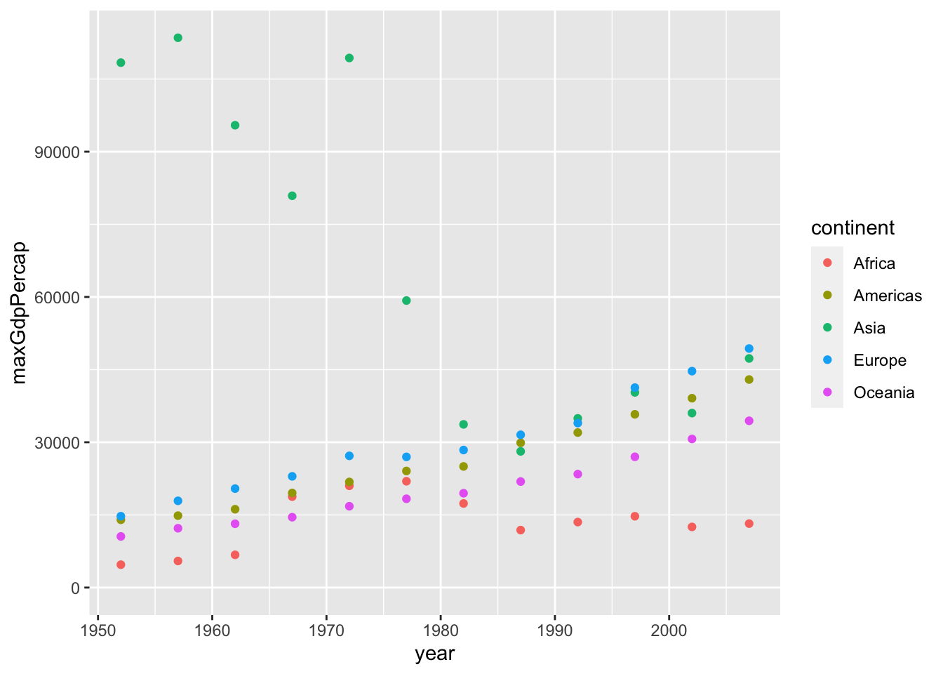
Examples:
# Summarize the median GDP and median life expectancy per continent in 2007
by_continent_2007 <- gapminder %>%
  filter(year == 2007) %>%
  group_by(continent) %>%
  summarize(medianGdpPercap = median(gdpPercap),
            medianLifeExp = median(lifeExp))
## `summarise()` ungrouping output (override with `.groups` argument)# Use a scatter plot to compare the median GDP and median life expectancy
ggplot(by_continent_2007, aes(x = medianGdpPercap, y = medianLifeExp, color = continent)) +
geom_point()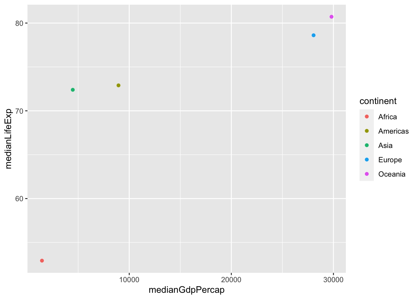
4.3 Types of visualizations
- Line Plots: Useful for showing change over time.
- Bar Plots: Good at comparing statistics for each of several categories
- Histogram: Describe the distribution of one dimensional numeric variable
- Box Plot : Compare the distribution of numeric variable over several categories.
Line Plots:
Change geom_point() to geom_line():
## `summarise()` ungrouping output (override with `.groups` argument)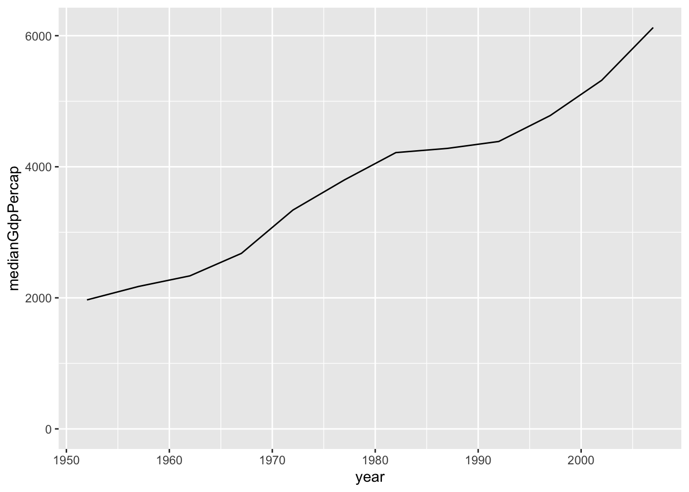
Example:
# Summarize the median gdpPercap by year & continent, save as by_year_continent
by_year_continent <- gapminder %>% group_by                         (continent, year) %>%
                        summarize(medianGdpPercap = median(gdpPercap))
## `summarise()` regrouping output by 'continent' (override with `.groups` argument)# Create a line plot showing the change in medianGdpPercap by continent over time
ggplot(by_year_continent, aes(x = year, y = medianGdpPercap, color = continent)) +
geom_line() +
expand_limits(y = 0)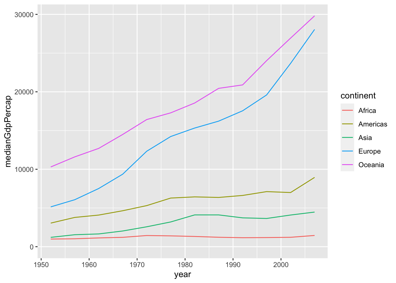
Bar Plots:
We use geom_col() for bar plots.
by_continent <- gapminder %>%
  filter(year == 1952) %>%
  group_by(continent) %>%
  summarize(medianGdpPercap = median(gdpPercap))
## `summarise()` ungrouping output (override with `.groups` argument)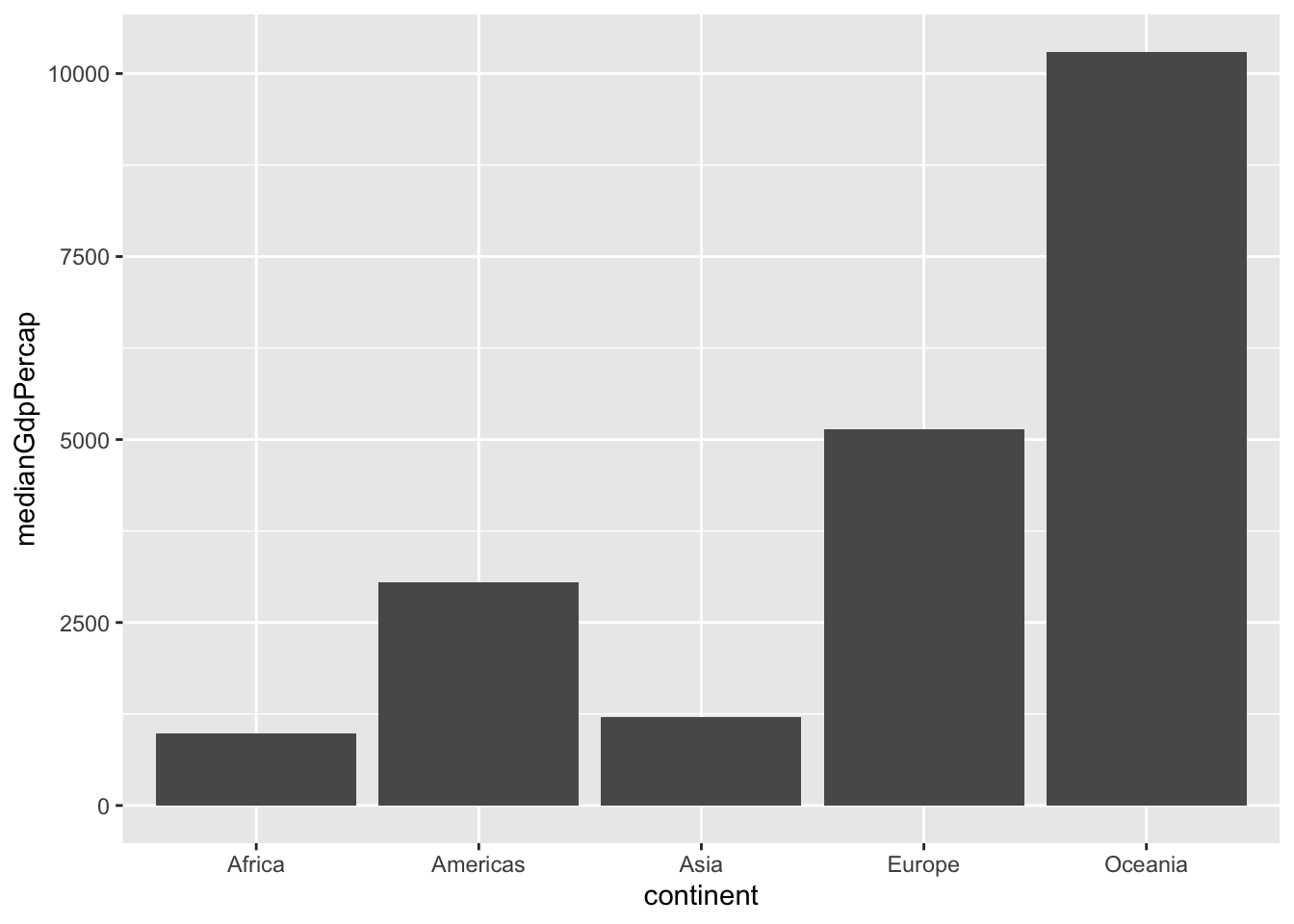
Histograms:
WE use geom_histogram() for histogram.Only one aesthetic. We can use binwidth to to change the width of each bar of a histogram. We can also use scale_x/y_log10 to make x axis or y axis more readable.
gapminder_1952 <- gapminder %>%
  filter(year == 1952) %>%
  mutate(pop_by_mil = pop / 1000000)

# Create a histogram of population (pop_by_mil)

ggplot(gapminder_1952, aes(x = pop_by_mil)) +
  geom_histogram(bins = 50) +
  scale_x_log10()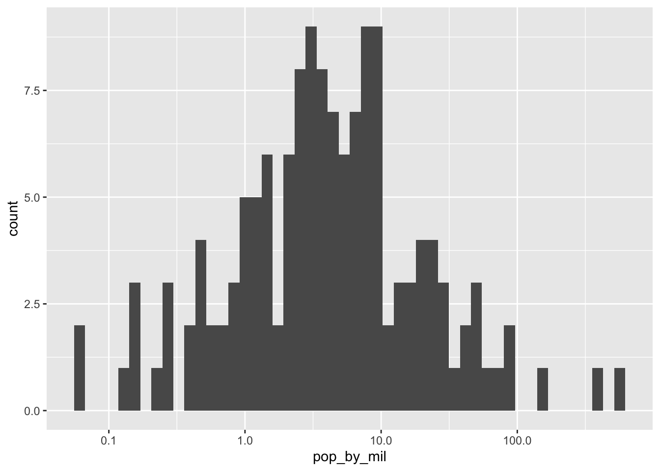
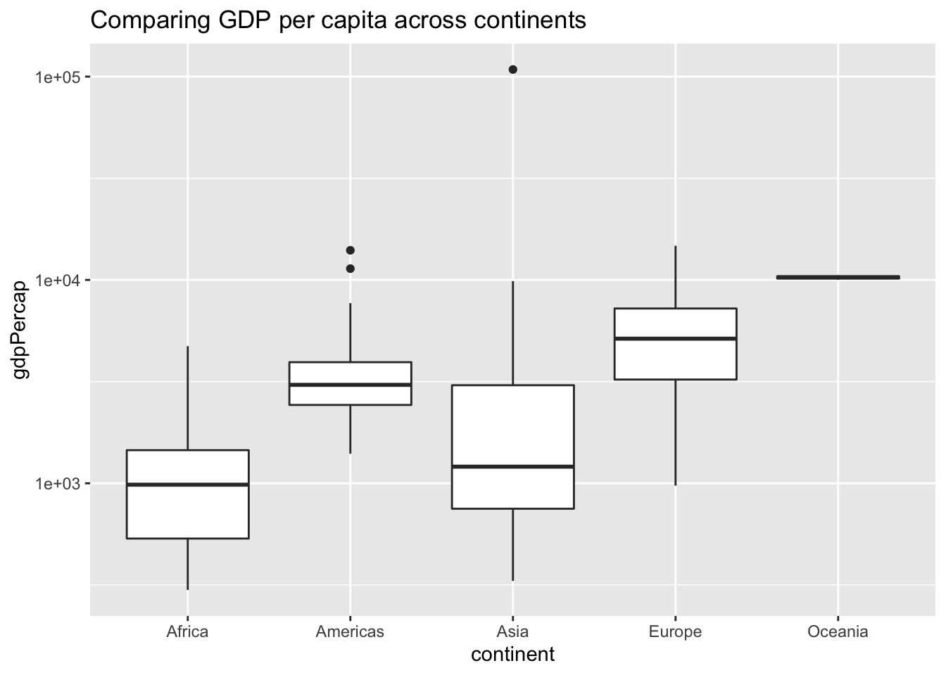
BoxPlot :
We use boxplots to compare numeric variables over several categories.
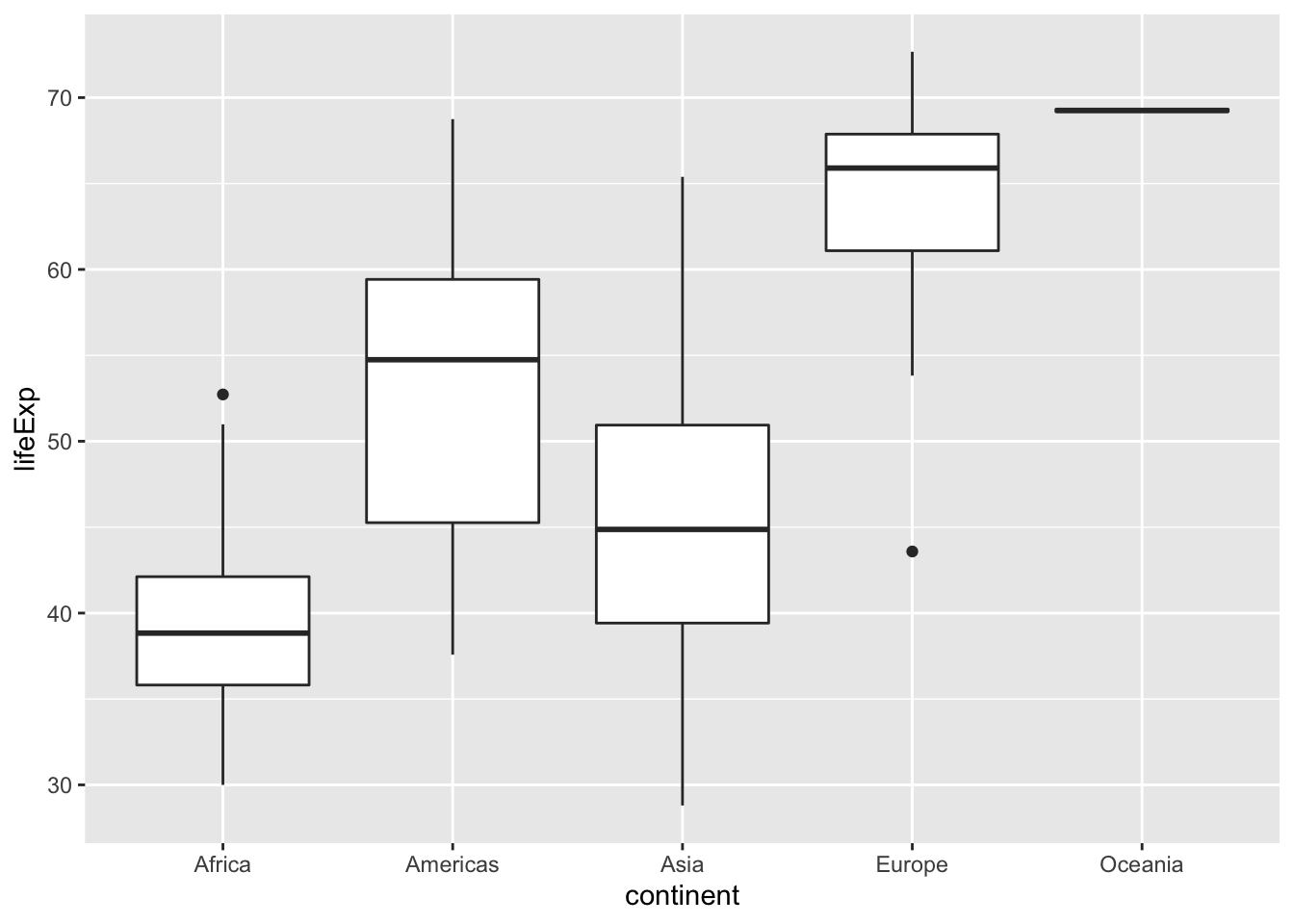
In order to add title to the graphs, we use :
ggtitle(“Title”) to the code. Example :
ggplot(gapminder_1952, aes(x = continent, y = gdpPercap)) +
  geom_boxplot() +
  scale_y_log10() +
  ggtitle("Comparing GDP per capita across continents")