7 Categorical Data in the Tidyverse
https://learn.datacamp.com/courses/categorical-data-in-the-tidyverse
##
## Attaching package: 'dplyr'
## The following objects are masked from 'package:stats':
##
## filter, lag## The following objects are masked from 'package:base':
##
## intersect, setdiff, setequal, union## ── Attaching packages ───────────────────────── tidyverse 1.3.0 ──## ✓ ggplot2 3.3.3 ✓ purrr 0.3.4
## ✓ tibble 3.0.3 ✓ stringr 1.4.0
## ✓ tidyr 1.1.2 ✓ forcats 0.5.0
## ✓ readr 1.3.1## ── Conflicts ──────────────────────────── tidyverse_conflicts() ──
## x dplyr::filter() masks stats::filter()
## x dplyr::lag() masks stats::lag()7.1 Introduction to Factor Variables
Categorical Data (Nominal): Categorical Data are the data that fall under un-ordered groups.Ex: Occupation
Ordinal Data(Qualitive): Have an inherit order but not a constant distance between them. Ex: Income (o-50k, 50k - 150k, 150k - 500k) <- there is an inherit order (smallest to largest) but no constant distance.
How do you know that a variable is factor or character?
## Some larger datasets need to be installed separately, like senators and
## house_district_forecast. To install these, we recommend you install the
## fivethirtyeightdata package by running:
## install.packages('fivethirtyeightdata', repos =
## 'https://fivethirtyeightdata.github.io/drat/', type = 'source')## # A tibble: 173 x 11
## major_code major major_category total employed employed_fullti… unemployed
## <int> <chr> <chr> <int> <int> <int> <int>
## 1 1100 Gene… Agriculture &… 128148 90245 74078 2423
## 2 1101 Agri… Agriculture &… 95326 76865 64240 2266
## 3 1102 Agri… Agriculture &… 33955 26321 22810 821
## 4 1103 Anim… Agriculture &… 103549 81177 64937 3619
## 5 1104 Food… Agriculture &… 24280 17281 12722 894
## 6 1105 Plan… Agriculture &… 79409 63043 51077 2070
## 7 1106 Soil… Agriculture &… 6586 4926 4042 264
## 8 1199 Misc… Agriculture &… 8549 6392 5074 261
## 9 1301 Envi… Biology & Lif… 106106 87602 65238 4736
## 10 1302 Fore… Agriculture &… 69447 48228 39613 2144
## # … with 163 more rows, and 4 more variables: unemployment_rate <dbl>,
## # p25th <dbl>, median <dbl>, p75th <dbl>## # A tibble: 6 x 11
## major_code major major_category total employed employed_fullti… unemployed
## <int> <chr> <chr> <int> <int> <int> <int>
## 1 1100 Gene… Agriculture &… 128148 90245 74078 2423
## 2 1101 Agri… Agriculture &… 95326 76865 64240 2266
## 3 1102 Agri… Agriculture &… 33955 26321 22810 821
## 4 1103 Anim… Agriculture &… 103549 81177 64937 3619
## 5 1104 Food… Agriculture &… 24280 17281 12722 894
## 6 1105 Plan… Agriculture &… 79409 63043 51077 2070
## # … with 4 more variables: unemployment_rate <dbl>, p25th <dbl>, median <dbl>,
## # p75th <dbl>## [1] FALSETo change all columns from characters to factors, we use:
levels() will gave us the name of factors and nlevels() will give us the number of levels of a factor.
## [1] 16## [1] "Agriculture & Natural Resources" "Arts"
## [3] "Biology & Life Science" "Business"
## [5] "Communications & Journalism" "Computers & Mathematics"
## [7] "Education" "Engineering"
## [9] "Health" "Humanities & Liberal Arts"
## [11] "Industrial Arts & Consumer Services" "Interdisciplinary"
## [13] "Law & Public Policy" "Physical Sciences"
## [15] "Psychology & Social Work" "Social Science"Summarising Factors:
## # A tibble: 1 x 2
##   major major_category
##   <int>          <int>
## 1   173             16
Top_n() and Pull()
dplyr has two other functions that can come in handy when exploring a dataset. The first is top_n(x, var), which gets us the first x rows of a dataset based on the value of var. The other is pull(), which allows us to extract a column and take out the name, leaving only the value(s) from the column.
## [1] Social Science Social Science Social Science Social Science Social Science
## [6] Social Science Social Science Social Science Social Science
## 16 Levels: Agriculture & Natural Resources Arts ... Social Science
college_all_ages %>%
# pull CurrentJobTitleSelect
pull(major_category) %>%
# get the values of the levels
levels()## [1] "Agriculture & Natural Resources" "Arts"
## [3] "Biology & Life Science" "Business"
## [5] "Communications & Journalism" "Computers & Mathematics"
## [7] "Education" "Engineering"
## [9] "Health" "Humanities & Liberal Arts"
## [11] "Industrial Arts & Consumer Services" "Interdisciplinary"
## [13] "Law & Public Policy" "Physical Sciences"
## [15] "Psychology & Social Work" "Social Science"Re-ordering Factors:
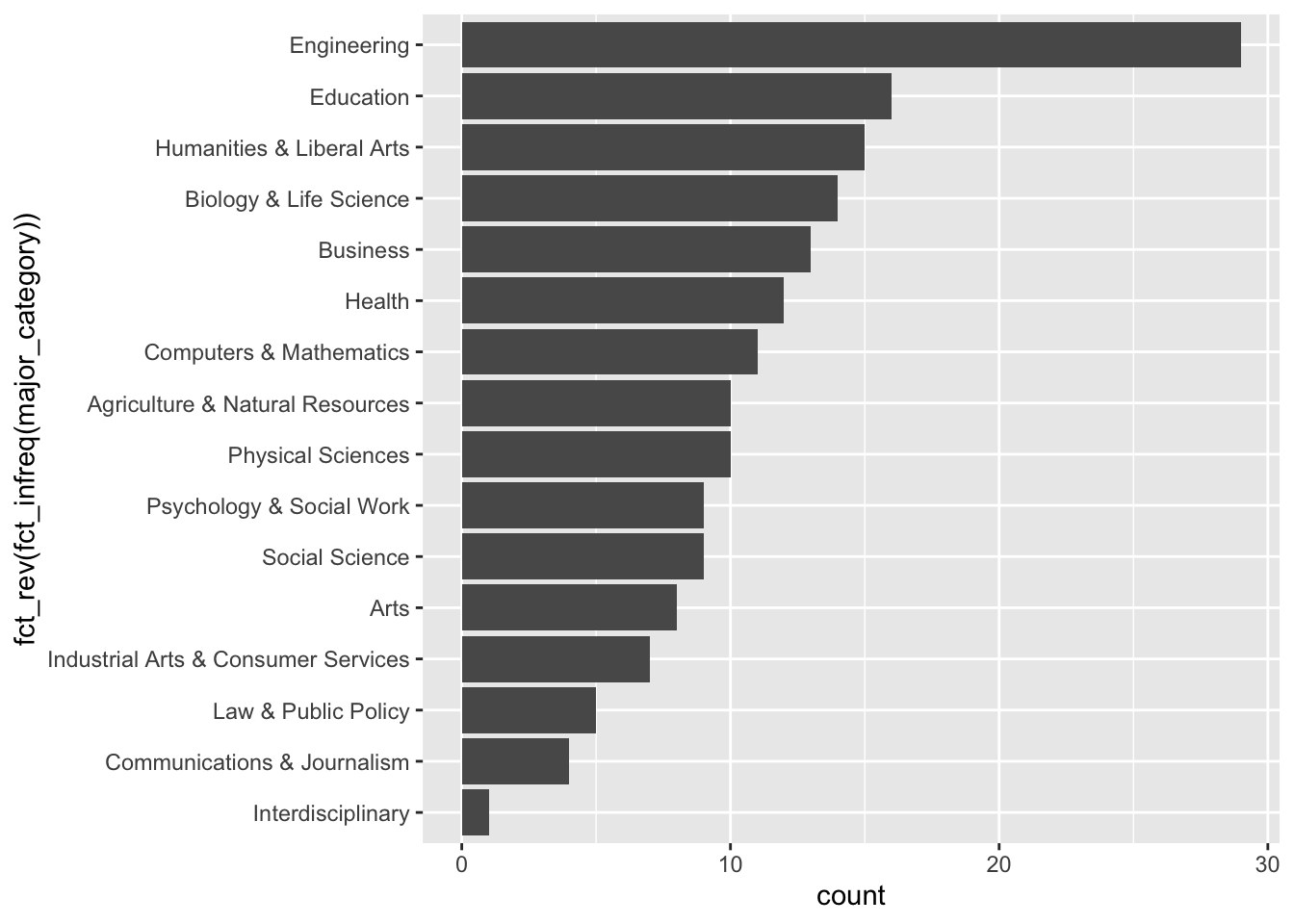
We can rearrange bar plots using the fct_infreq() function:
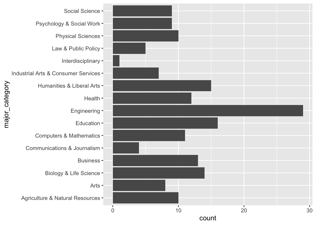
college_all_ages%>%
  # remove NAs
  filter(!is.na(major_category) & !is.na(employed)) %>%
  # get mean_employed by major_category
  group_by(major_category) %>%
  summarise(mean_employed = mean(employed)) %>%
  # reorder major_category by mean_employed
  mutate(major_category = fct_reorder(major_category, mean_employed)) %>%
  # make a scatterplot of major_category by mean_employed
  ggplot(aes(x = major_category, y = mean_employed)) +
    geom_point() +
    coord_flip()
## `summarise()` ungrouping output (override with `.groups` argument)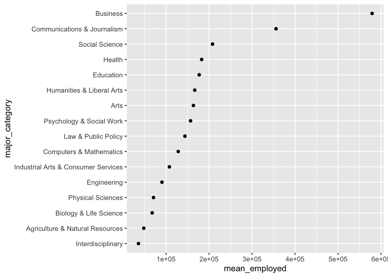
7.2 Manipulating Factor Variables
We can use fct_relevel to reorder the x axis.
multiple_choice_responses %>%
# Move "I did not complete any formal education past high school" and "Some college/university study without earning a bachelor's degree" to the frontmutate(FormalEducation = fct_relevel(FormalEducation, “I did not complete any formal education past high school”, “Some college/university study without earning a bachelor’s degree”)) %>%
# Move "I prefer not to answer" to be the last level.mutate(FormalEducation = fct_relevel(FormalEducation, “I prefer not to answer”, after = Inf)) %>%
# Move "Doctoral degree" to be after the 5th levelmutate(FormalEducation = fct_relevel(FormalEducation, “Doctoral degree”, after = 5)) %>%
# Examine the new level orderpull(FormalEducation) %>% levels()
Renaming Factor Levels:
Sometimes we need to change the names of certain observations in a variable as the names are too long.
We can do this by :
majorCategory_shortform <- college_all_ages %>% mutate(major_shortform = fct_recode(major_category,
                          "A&R" = "Agriculture & Resources ",
                          "B&LS" = "Biology & Life Science",
                          "A&NS" = "Agriculture & Natural Resources"))
## Warning: Problem with `mutate()` input `major_shortform`.
## ℹ Unknown levels in `f`: Agriculture & Resources
## ℹ Input `major_shortform` is `fct_recode(...)`.## Warning: Unknown levels in `f`: Agriculture & Resources## # A tibble: 1 x 2
## `nlevels(major_category)` n
## <int> <int>
## 1 16 173We can use fct_collapse to make a new level that is a combination of other levels. We can also use the fct_other() and fct_keep().
Example Code:
multiple_choice_responses %>%
# Create new variable, grouped_titles, by collapsing levels in CurrentJobTitleSelect
mutate(grouped_titles = fct_collapse(CurrentJobTitleSelect,
    "Computer Scientist" = c("Programmer", "Software Developer/Software Engineer"),
    "Researcher" = "Scientist/Researcher",
    "Data Analyst/Scientist/Engineer" = c("DBA/Database Engineer", "Data Scientist",
                                      "Business Analyst", "Data Analyst",
                                      "Data Miner", "Predictive Modeler"))) %>%

# Keep all the new titles and turn every other title into "Other"
mutate(grouped_titles = fct_other(grouped_titles,
                                  keep = c("Computer Scientist",
                                           "Researcher",
                                           "Data Analyst/Scientist/Engineer"))) %>%

# Get a count of the grouped titles
count(grouped_titles)

  # remove NAs of MLMethodNextYearSelect
filter(!is.na(MLMethodNextYearSelect)) %>%
# create ml_method, which lumps all those with less than 5% of people into "Other"mutate(ml_method = fct_lump(MLMethodNextYearSelect, prop = .05)) %>%
# count the frequency of your new variable, sorted in descending ordercount(ml_method, sort = TRUE)
7.3 Creating Factor Variables
We can use the if_else statement a mutate function:
college_all_ages %>%
    # If usefulness is "Not Useful", make 0, else 1
    mutate(Agriculture = if_else(major_category == "Agriculture & Natural Resources", "Yes", "No")) %>% count(Agriculture == "Yes")
## # A tibble: 2 x 2
## `Agriculture == "Yes"` n
## <lgl> <int>
## 1 FALSE 163
## 2 TRUE 10Tricks of ggplot2
Change tick labels angle: If the names in the x axis are too long and overlap, we can use the angle of the names to 90 degrees using the theme(axis.text.x = element_text(angle = 90, hjust = 1))
college_all_ages%>%
# remove NAs
filter(!is.na(major_category) & !is.na(employed)) %>%
# get mean_employed by major_category
group_by(major_category) %>%
summarise(mean_employed = mean(employed)) %>%
# reorder major_category by mean_employed
mutate(major_category = fct_reorder(major_category, mean_employed)) %>%
# make a scatterplot of major_category by mean_employed
ggplot(aes(x = major_category, y = mean_employed)) +
geom_point() +
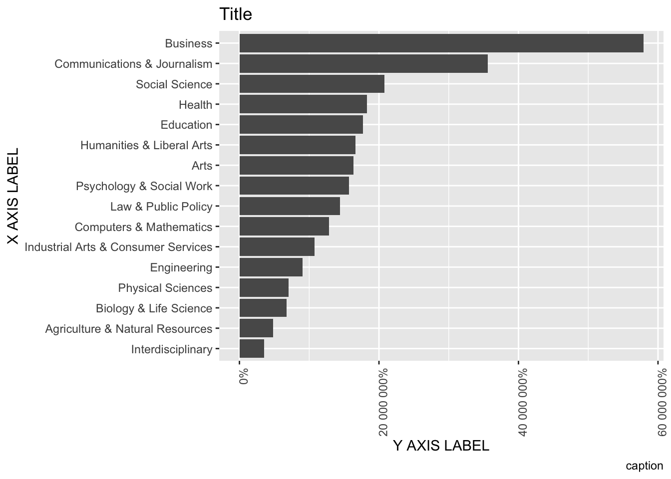
theme(axis.text.x = element_text(angle = 90, hjust = 1))## `summarise()` ungrouping output (override with `.groups` argument)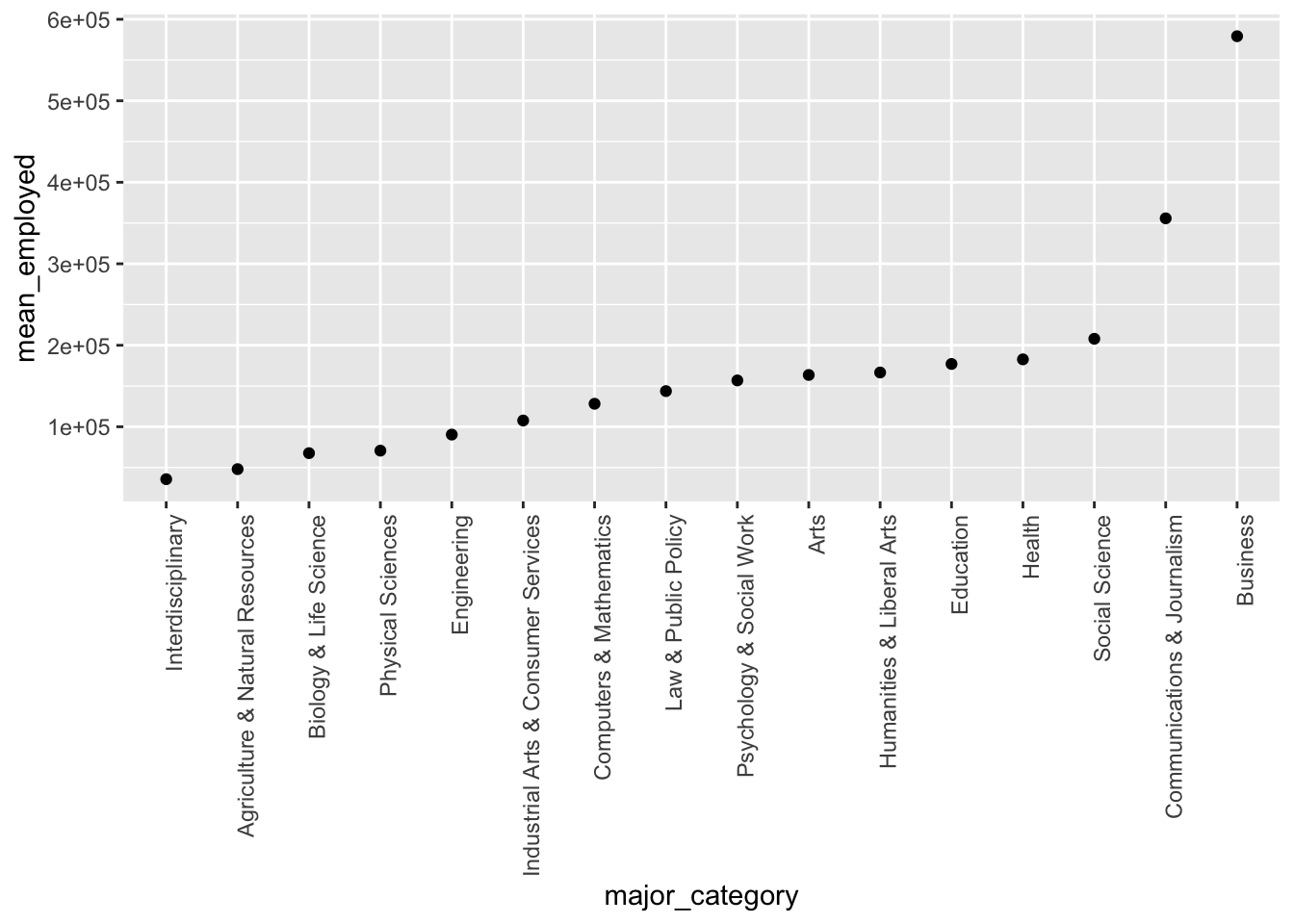 WE use labs() to change labels and the scale_y_continous() function to change an axis to percentage.
college_all_ages%>%
  # remove NAs
  filter(!is.na(major_category) & !is.na(employed)) %>%
  # get mean_employed by major_category
  group_by(major_category) %>%
  summarise(mean_employed = mean(employed)) %>%
  # reorder major_category by mean_employed
  mutate(major_category = fct_reorder(major_category, mean_employed)) %>%
  # make a scatterplot of major_category by mean_employed
  ggplot(aes(x = major_category, y = mean_employed)) +
    geom_point() +
  theme(axis.text.x = element_text(angle = 90, hjust = 1)) +
  labs(x = "X AXIS LABEL", y = "Y AXIS LABEL") +
    scale_y_continuous(labels = scales::percent)
## `summarise()` ungrouping output (override with `.groups` argument)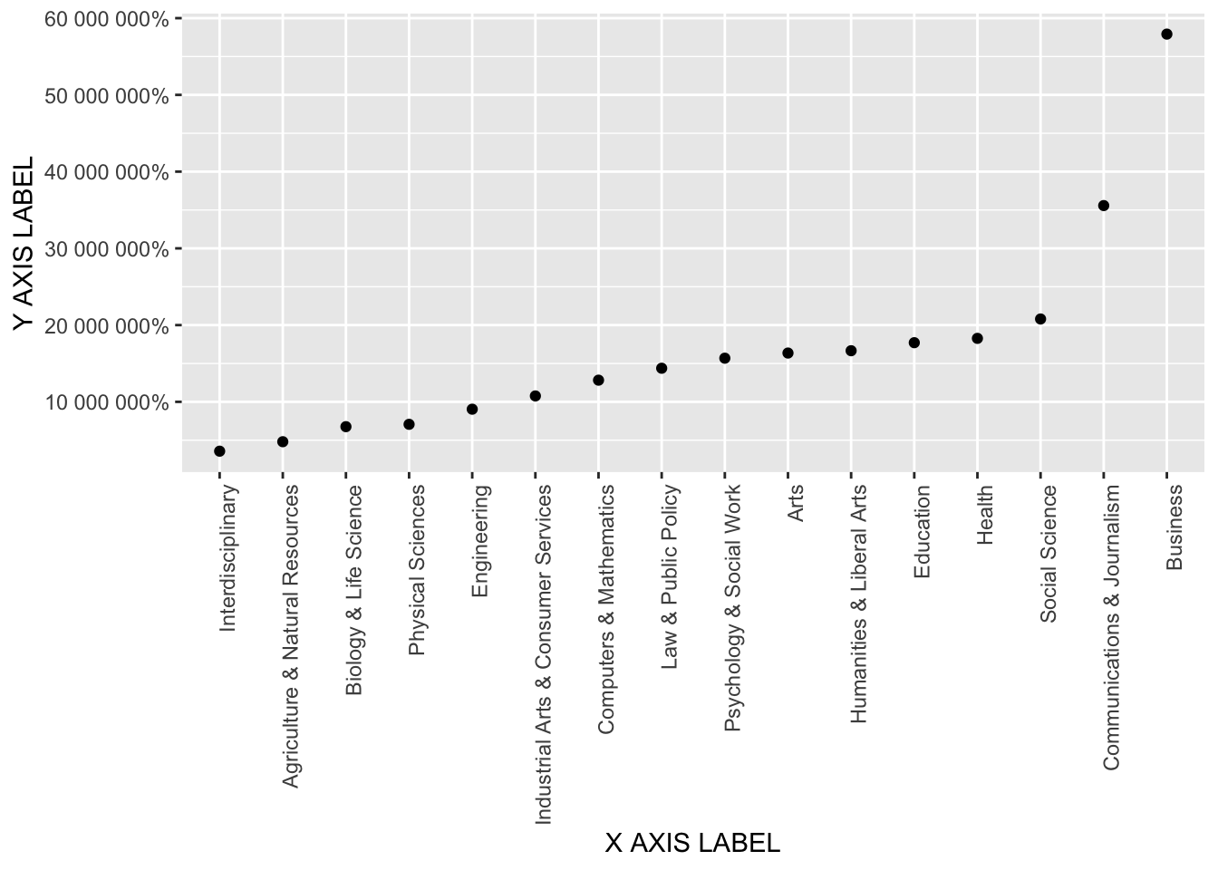
Changing and creating Variables with case_when():
c <- 1:20
case_when(c %% 15 == 0 ~ "Divisible by 15",
          c %% 3 == 0 ~ "Divisible by 3",
          c %% 2 == 0 ~ "Divisible by 2",
          TRUE ~ "Not divisible by 3/15")
## [1] "Not divisible by 3/15" "Divisible by 2" "Divisible by 3"
## [4] "Divisible by 2" "Not divisible by 3/15" "Divisible by 3"
## [7] "Not divisible by 3/15" "Divisible by 2" "Divisible by 3"
## [10] "Divisible by 2" "Not divisible by 3/15" "Divisible by 3"
## [13] "Not divisible by 3/15" "Divisible by 2" "Divisible by 15"
## [16] "Divisible by 2" "Not divisible by 3/15" "Divisible by 3"
## [19] "Not divisible by 3/15" "Divisible by 2"7.4 Case Study on Flight Etiquette
We can use Regex to find instances of general patterns. WE use the str_detect() function. The “.” matches any character. The "*" says match the chararcter before me 0 or more times.
## [1] TRUE## [1] TRUE## [1] FALSETo remove anything up to "*" we use str_remove():
## [1] " best"We can add titles, subtitle, caption and labels to a graph:
#Summary:
forcats funcitons:
% fct_reorder(), fct_collapse(), fct_other(), fct_relevel(), fct_rev(), & fct_recode()
college_all_ages%>%
  # remove NAs
  filter(!is.na(major_category) & !is.na(employed)) %>%
  # get mean_employed by major_category
  group_by(major_category) %>%
  summarise(mean_employed = mean(employed)) %>%
  # reorder major_category by mean_employed
  mutate(major_category = fct_reorder(major_category, mean_employed))
## `summarise()` ungrouping output (override with `.groups` argument)## # A tibble: 16 x 2
## major_category mean_employed
## <fct> <dbl>
## 1 Agriculture & Natural Resources 48042.
## 2 Arts 163587.
## 3 Biology & Life Science 67647
## 4 Business 579219.
## 5 Communications & Journalism 355760.
## 6 Computers & Mathematics 128237
## 7 Education 177075.
## 8 Engineering 90413.
## 9 Health 182724.
## 10 Humanities & Liberal Arts 166612.
## 11 Industrial Arts & Consumer Services 107683.
## 12 Interdisciplinary 35706
## 13 Law & Public Policy 143785.
## 14 Physical Sciences 70713.
## 15 Psychology & Social Work 156887
## 16 Social Science 207978.college_all_ages %>%
select(-employed_fulltime_yearround, -unemployment_rate, -p25th, -median, -p75th, -major, -major_code) %>%
# Create new variable, grouped_titles, by collapsing levels in CurrentJobTitleSelect
mutate(grouped_majors = fct_collapse(major_category,
"Agriculture" = "Agriculture & Natural Resources")) %>%
# Keep all the new titles and turn every other title into "Other"
mutate(grouped_majors = fct_other(grouped_majors,
keep = c("Agriculture")))## # A tibble: 173 x 5
## major_category total employed unemployed grouped_majors
## <fct> <int> <int> <int> <fct>
## 1 Agriculture & Natural Resources 128148 90245 2423 Agriculture
## 2 Agriculture & Natural Resources 95326 76865 2266 Agriculture
## 3 Agriculture & Natural Resources 33955 26321 821 Agriculture
## 4 Agriculture & Natural Resources 103549 81177 3619 Agriculture
## 5 Agriculture & Natural Resources 24280 17281 894 Agriculture
## 6 Agriculture & Natural Resources 79409 63043 2070 Agriculture
## 7 Agriculture & Natural Resources 6586 4926 264 Agriculture
## 8 Agriculture & Natural Resources 8549 6392 261 Agriculture
## 9 Biology & Life Science 106106 87602 4736 Other
## 10 Agriculture & Natural Resources 69447 48228 2144 Agriculture
## # … with 163 more rowsmajorCategory_shortform <- college_all_ages %>%
select(-employed_fulltime_yearround, -unemployment_rate, -p25th, -median, -p75th, -major, -major_code) %>%
mutate(major_shortform = fct_recode(major_category,
"A&R" = "Agriculture & Resources ",
"B&LS" = "Biology & Life Science",
"A&NS" = "Agriculture & Natural Resources"))## Warning: Problem with `mutate()` input `major_shortform`.
## ℹ Unknown levels in `f`: Agriculture & Resources
## ℹ Input `major_shortform` is `fct_recode(...)`.## Warning: Unknown levels in `f`: Agriculture & Resources## # A tibble: 173 x 5
## major_category total employed unemployed major_shortform
## <fct> <int> <int> <int> <fct>
## 1 Agriculture & Natural Resources 128148 90245 2423 A&NS
## 2 Agriculture & Natural Resources 95326 76865 2266 A&NS
## 3 Agriculture & Natural Resources 33955 26321 821 A&NS
## 4 Agriculture & Natural Resources 103549 81177 3619 A&NS
## 5 Agriculture & Natural Resources 24280 17281 894 A&NS
## 6 Agriculture & Natural Resources 79409 63043 2070 A&NS
## 7 Agriculture & Natural Resources 6586 4926 264 A&NS
## 8 Agriculture & Natural Resources 8549 6392 261 A&NS
## 9 Biology & Life Science 106106 87602 4736 B&LS
## 10 Agriculture & Natural Resources 69447 48228 2144 A&NS
## # … with 163 more rowstidyverse functions:
% case_when(), mutate_if(), gather(), & str_remove()
c <- 1:20
case_when(c %% 15 == 0 ~ "Divisible by 15",
          c %% 3 == 0 ~ "Divisible by 3",
          c %% 2 == 0 ~ "Divisible by 2",
          TRUE ~ "Not divisible by 3/15")
## [1] "Not divisible by 3/15" "Divisible by 2" "Divisible by 3"
## [4] "Divisible by 2" "Not divisible by 3/15" "Divisible by 3"
## [7] "Not divisible by 3/15" "Divisible by 2" "Divisible by 3"
## [10] "Divisible by 2" "Not divisible by 3/15" "Divisible by 3"
## [13] "Not divisible by 3/15" "Divisible by 2" "Divisible by 15"
## [16] "Divisible by 2" "Not divisible by 3/15" "Divisible by 3"
## [19] "Not divisible by 3/15" "Divisible by 2"## [1] " best"ggplot2 tricks:
% scales :: percent_format(), labs(), & axis.text.x
college_all_ages%>%
  # remove NAs
  filter(!is.na(major_category) & !is.na(employed)) %>%
  # get mean_employed by major_category
  group_by(major_category) %>%
  summarise(mean_employed = mean(employed)) %>%
  # reorder major_category by mean_employed
  mutate(major_category = fct_reorder(major_category, mean_employed)) %>%
  # make a scatterplot of major_category by mean_employed
  ggplot(aes(x = major_category, y = mean_employed)) +
    geom_col() +
  theme(axis.text.x = element_text(angle = 90, hjust = 1)) +
  labs(x = "X AXIS LABEL", y = "Y AXIS LABEL", title = "Title", caption = "caption") +
    scale_y_continuous(labels = scales::percent) +
  coord_flip()
## `summarise()` ungrouping output (override with `.groups` argument)