3.1 Category 1 Variable 1: Median Income, which measure the average income of the past 12 months within each county.

3.1.1 Map of Median Income in the United States

my.bins <- c(0, 10000, 20000, 25000, 30000, 35000, 40000,45000,50000,75000)
pal <- colorBin("Greens", metadataGIS$median_income, bins = my.bins, reverse=FALSE)

leaflet(metadataGIS, options = leafletOptions(crsClass = "L.CRS.EPSG3857"), width="100%") %>%
  addPolygons(weight = 0.5, color = "white", opacity = 0.7,
    fillColor = ~pal(median_income), fillOpacity = 1, smoothFactor = 0.5,
    label = popupPlus("Median Income", metadataGIS$median_income, "number"),
    labelOptions = labelOptions(direction = "auto")) %>%
    addPolygons(data = stateGIS,fill = FALSE,color="black",weight = 1) %>%
    addLegend(pal = pal,values = ~metadataGIS$median_income, opacity = 1, title = "Median Income",position = "bottomright")

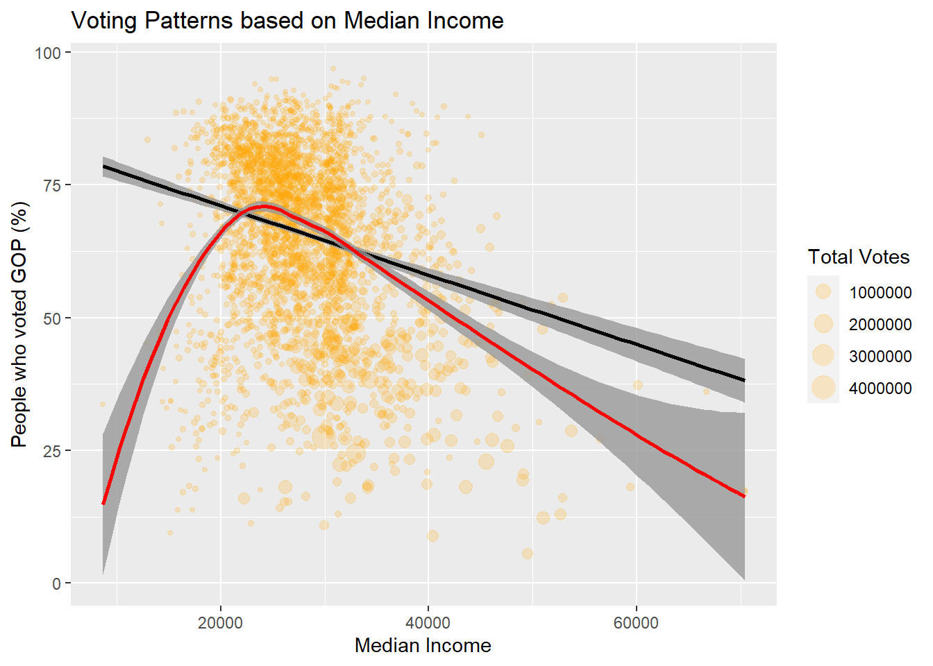
3.1.2 Scatterplot of Median Income and % of GOP Votes in a county

ggplot(metadata,aes(x=median_income,y=pctGOP*100, size=totalVotes))+
  geom_point(alpha=.2,color="Orange")+
  geom_smooth(method="lm",color="Black",alpha=.8, show.legend = FALSE)+
  geom_smooth(method="loess",color="red",alpha=.8, show.legend = FALSE)+
  labs(title="Voting Patterns based on Median Income",x="Median Income",y="People who voted GOP (%)",
       size = "Total Votes")

3.1.3 Summary Table for Regression of Median Income

model4.1<-lm(pctGOP~median_income,data=metadata)
stargazer(model4.1, 
          type = "html", 
          report=('vc*p'),
          keep.stat = c("n","rsq","adj.rsq"), 
          notes = "<em>&#42;p&lt;0.1;&#42;&#42;p&lt;0.05;&#42;&#42;&#42;p&lt;0.01</em>", 
          notes.append = FALSE)


	Dependent variable:

	pctGOP

median_income	-0.00001^***
	p = 0.000

Constant	0.841^***
	p = 0.000


Observations	3,108
R²	0.055
Adjusted R²	0.055

Note:	p<0.1;p<0.05;**p<0.01